LOGISTICS ROBOT IN WAREHOUSE

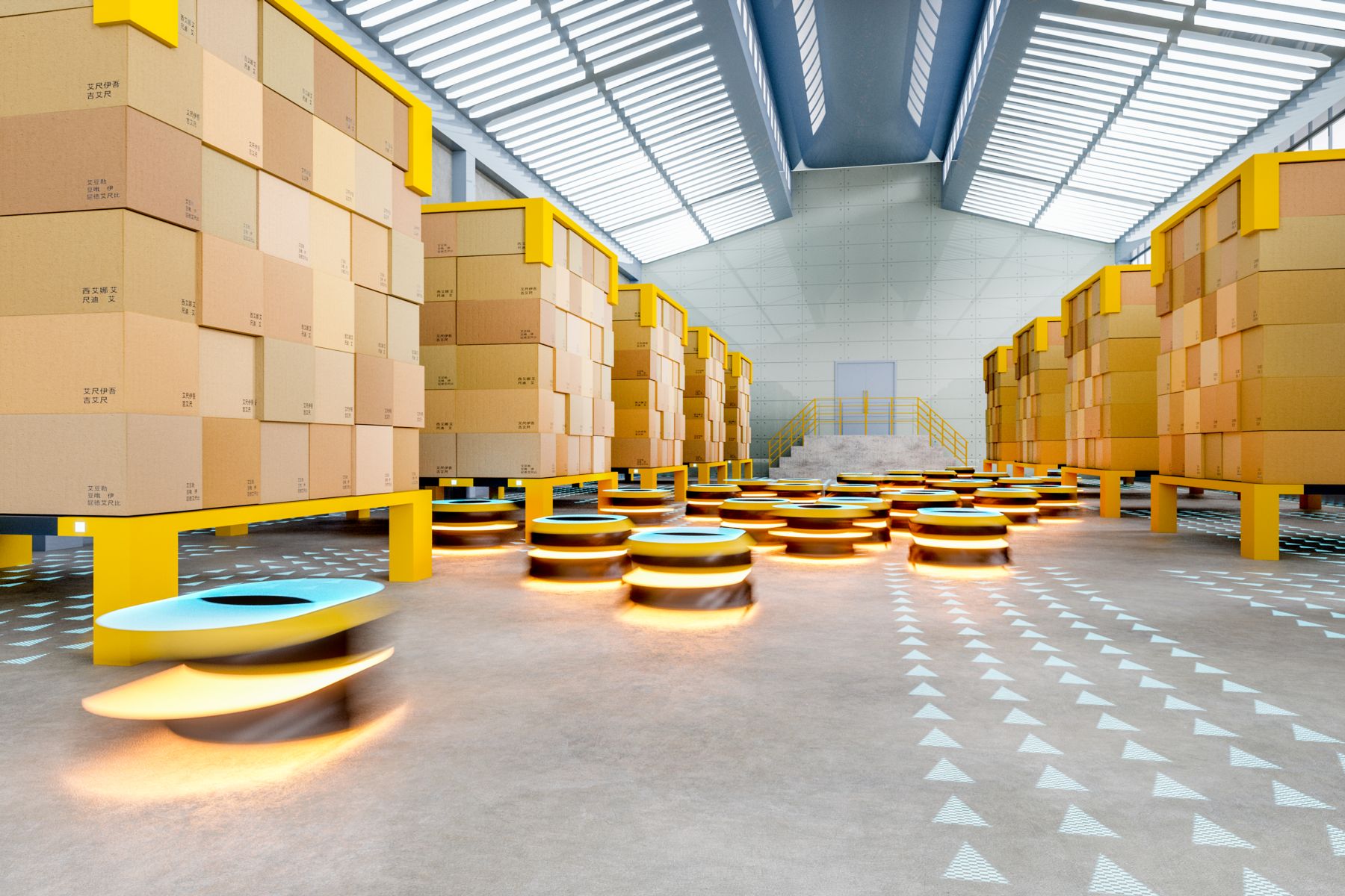
The goal of this project is to configure and program a logistics robot that is moving inside a Warehouse, moving shelves from a specific location to a required new location. The robot should be able to approach to the shelve that needs to be transferred, locate below it, and move it to the new location following the shortest path possible. In order to do this, it will need to understand the environment (Warehouse map), the holonomic restrictions depending if its holding a shelve or not and his specific location inside the map. The aim of this project is also to apply the OMPL library and its functionalities in order to resolve the problem.

General Outline

The problem that we need to solve can be divided in different sub-problems or states. These are: approach the robot to the shelve that needs to transport, lift his platform and pick it up, move to the goal position and put down the shelve. For the localization of the robot, we will use the warehouse map to transform the coordinates of the robot (given by the API, in the 3D World) to the 2D coordinates in the map image (pixel coordinates), as we did in the first project. For the navigation/movement algorithm, we will use the OMPL library to handle all the complexity of movement restrictions, path planning, etc... 

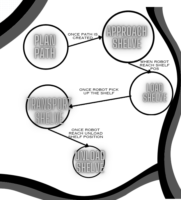
Here is the outline of the Finite State Machine (FSM) suggested for the resolution of this exercise:

Also, as we did in previous exercises [1] [2], [3], all the functions for the movement and control of the robot will be managed by a custom class for it: LogisticsRobot class.

First step: Localization in the warehouse map

The API give us the coordinates (x,y) of the logistics robot in the 3D world, but all the logic and intelligence of the robot will be interpret towards the warehouse map. Therefore, we need to transform that coordinates system to the correspondence position in the 2D warehouse map.

In order to do this, we will choose a number of points in the 3D world and the (approximated) correspondent pixel in the 2D map and we will compute the best fitting regression line to do this transformation between coordinates. For this samples, we will take points that are a little bit distant between them to reduce the error. The best option is to take corner points and the origin point of the Gazebo world:

After some measures, we have the following regression line:

This is the mathematical expression in form of y = b + m*x

With this we already have a mechanism to manage the coordinates of the logistics robot and the shelves we need to transport. To keep the things simple, I also turn the map in grayscale with only black and white values (obstacles and free positions). Also, an erosion was made to augment the obstacles a little bit, avoiding problems in the following steps related with planning and navigation.

Second step: Path planning of the robot to approach to shelves. OMPL

The robot will need to approach to the shelves moving through the map without hitting obstacles and in the most efficient and short path possible. In this sub-state, the robot will be considered holonomic as it doesn't have the shelves in top of him, so there are no restrictions in the movement.  In order to do this planning step, we will use OMPL (Open Motion Planning Library):

"OMPL is an open-source software library designed to facilitate motion planning for robotic systems. Motion planning involves determining a feasible path for a robot to move from its current state to a desired goal state, avoiding obstacles and taking into account the robot's dynamics and constraints"

The OMPL structure is made up by many important components. We will focus on the following ones, applying the also the mentioned configuration:

• State Space: Defines the possible configurations of the robot (Euclidean Space, SO2, SE2, SE3...). For our case, we have a Euclidean Space.

• State Validaty Checker: Determines if the configuration is valid (this is, that it doesn't collides with an enviroment obstacle and respects the constraints of the robot). For a first approximation, we will consider a valid state if it is not an obstacle.

• Planner: Responsible for generating the path from the start to the goal in the configuration space. OMPL offers many state-of-the-art planning algorithms such as PRM, RRT or KPIECE: For the first approximation, we will use RRT Connect
  

• Path: sequence of states representing a trajectory for the robot to follow. The path involves the sub-sequence of states (pixels/points) the robot should follow to reach the goal position (shelve position)

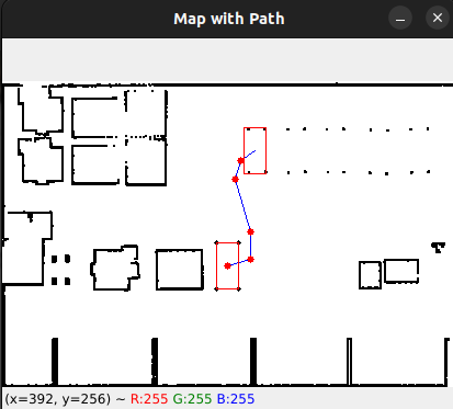
In the following images we can see the result of applying this first approximation (remember we are using RRT Connect as planner):

• The robot is being considered as a single point (single pixel). We should approach the robot to the real dimensions to avoid generating paths that goes to close to obstacles (see Figure 1, where robot is getting to close to a shelve leg).

• The RRT is not generating sometimes an efficient path (Paths of figures 1 and 3 are less efficient than path from figure 2, while figure 3 seems to be the most efficient path generated).

The Warehouse map dimensions are 20,62m (Width) x 13,60m (Height). The image dimensions are 414x278(pixels). This means that, if we consider the robot a single point (single pixel), we are considering the robot as dimensions 0.05x0.05meters (5cmx5cm, which is too far from reality). Taking in count the approximated squared form of the robot, and that is length is approximately something less than the length in x axis of the shelves, we can approach the robot to a square of NxN pixels in the map (this would be LxL meters in the real world, which is more realistic than the first approximation). The new dimension of the robot is defined by the constant ROBOT_DEFAULT_DIM.

Second Improvement: Optimize RRT Connect

In the previous executions of the code we saw that RRT sometimes didn't generate the best path to reach the goal. The RRT algorithm can be optimized not using the default max range between sub-states generated. With default value, the planner was generating always 1-2 sub-states between current position and goal. Changing this parameter can increase the execution time, but also increase the efficiency of the algorithm, as we have more sub-states, the path would increase the substates, must will be shortest in total distance for the robot.

Here is the next executions after applying both improvements in the code, as well as editing the drawing of the path to see the sub-states generated by the planner (click in the images to zoom):

As we can see, now the planner is generating always an efficient path to reach the goal position, and the number of sub-states have increased from 1-2 to 6-7.

Testing other planners

Before going to the step to generate the movement of the robot based on the path generated by the OMPL planner, we should test another planners to see if it exist other planners better than RRT Connect. OMPL contains a lot of planners availables:

• Probabilistic Road Map (PRM): Uses one thread to construct a roadmap while a second thread checks whether a path exists in the roadmap between a start and goal state. OMPL contains a number of variants of PRM.
  

For the initial position of the robot, PRM generates always the same path (Figure 1). For further distances, PRM can generate different paths, but all of them maintains its efficiency and keeps the geometry basics of the problem (Figures 2, 3 and 4).

• Informed RRT*: A variant of RRT* that uses heuristics to bound the search for optimal solutions. It uses the general cost framework.

For the initial position of the robot, Informed RRT* generates always the same path (Figure 1). For further distances, generates similar and efficient paths (Figures 2, 3 and 4). In relation with previous RRT, no need of modifying the max distance param is needed in this case.

• Batch Informed Tree (BIT*): An anytime asymptotically optimal algorithm that uses heuristics to order and bound the search for optimal solutions. It uses the general cost framework.

For the initial position of the robot, BIT* generates always the same path (Figure 1). For further distances, keeps generating similar and efficient paths, these with a large numer of sub-states (Figures 2, 3 and 4).

"After testing different planners, we can see that PRM and Informed RRT* can be good solutions to solve the problem, as they generate reduced number of sub-states in the path, Also, they keep always a particular same solution for short problems (short distance between init and goal)."

All the planning system for the 2D environment has been encapsulated in a class, Plane2DEnvironment, with the corresponding methods to create the plan, update the map at any point needed and other methods for plotting the path solution, getting the path points, etc...

Third step: Navigation to approach to shelve and pick it up

Once we have the path to reach the goal, its time to create a navigation system. The most simple idea is to re-use the same we did in the Global Navigation Exercise of the last year, creating a relative coordinates system of the next goal state (pixel) with respect the robot. This relative coordinates follows the SO2 OMPL State Space, that we got also in the planner solution. Then we can:

• Control lineal velocity of the robot based on the real distance between the current position and the goal position.

• Control angular velocity based on the robot yaw and the reference/desired angle to reach the goal.

Applying this, the robot didn't have a smooth navigation, mainly due to the constant big corrections with the angular velocity. Also, the linear velocity was too big, so I decided to apply a PD Controller to both velocities. As we did in previous exercises, I created the PDController class in order to do it. After applying the controller, the robot takes a smooth control, following all the path correctly and reaching the goal point successfully:

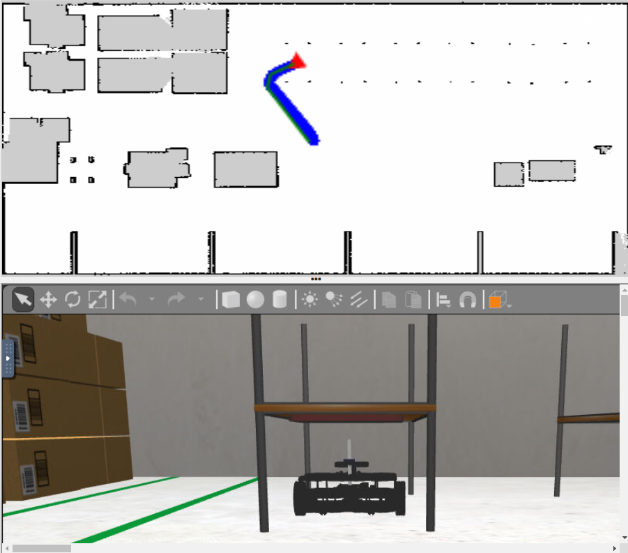
Notice that the robot is a little bit smaller than the width of the shelve, so it could enter to the bottom of the shelve directly and no by the sides, but I wanted to leave a bigger margin between the robot and the obstacles, so I expand a little bit the size of the robot (this is, the ROBOT_DEFAULT_DIM) of the robot. That's why, in the previous image, the planner choose the left side of the shelve to enter (it could be also the right side).

Once the robot reaches the goal position, I align his orientation with the desired orientated we told the planner in the plan() call parameters. As it is obvious, there is a small error margin in the yaw orientation for this step (YAW_ERROR_MARGIN), as well as another small error margin for the distance of reaching the goal positions (DIST_ERROR_MARGIN).

Once the robot is aligned with the goal yaw, we will lift the platform calling the lift method of the robot class. In a real world application this lift operation could take a few seconds, since the elevator has a specific velocity v and a distance Δy (Δt = Δy / v). To get an approximated solution taking in count this, we will wait that Δt (specified as LIFTING_TIME) before the robot starts the next step.

Fourth step: Transporting the shelve to the unloading place

After picking up the shelve, we need to carry it to the unloading place. To do this step, we just simply need to perform again the OMPL planning step and then navigate through the points till we reach the final point, but there is a couple of things we need to change now:

• The form of the robot has changed. Now, the shape is not a square of pixels as we specified in the ROBOT_DEFAULT_DIM constant, but it is of the same shape as the shelve is carrying out. The dimensions of the shelve had been taking approximated by the map image and are specified in the SHELVE_DIM constant (the new dimension of the robot during this step that will be taken in count during the new path planning).
• The shelve that is carrying out the robot is no longer part of the map obstacles. The map should be updated, removing the shelve legs of the map, that were previous obstacles.
  

In order to do this, I just made the following changes:

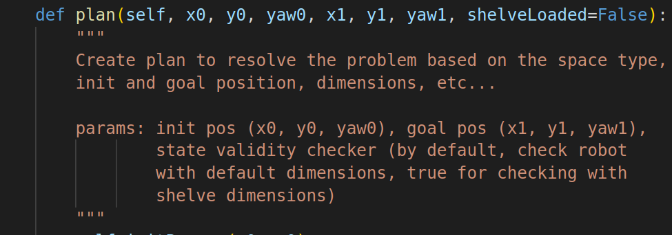
• plane() method of Plane2DEnvironment now takes as parameter the validity check function we want to use. Two different validity functions have been created, one of them takes in count the dimensions of the robot without the shelve (ROBOT_DEFAULT_DIM), and the other one takes in count the dimensions of the shelve itself (SHELVE_DIM):

• Created the functions removeShelve() and addShelve() to easily remove or add moved shelves on the map, updating their positions. This functions are not part of Plane2DEnvironment, so updateMap() method of this class should be call every time we update the map geometry and before executing another planner. Here's an example of using this classes to simulate the movement of the first shelve to a specific unloading position:

Last step: Unload shelve and repeat steps:

Once we check we have reached the unloading place for the shelve we are carrying, we call the putdown() method to unload the shelve, leaving again a specific LIFTING_TIME seconds to simulate the lift movement duration as in a real application. After this time, we would update our counter of moved shelves and, if there is still more shelves to move, we will repeat again the previous steps:

1. Plan the path to move the robot (using default geometry, robot is not transporting now a shelve) to the position of the next shelve we want to move.
2. Follow the path using the navigation system as before.
3. Once we reach the next shelve, pick it up, plan the path to reach the corresponding unloading place (using now the shelve geometry) and navigate through it. After reaching that location, we unload the shelve as mentioned in this section.
   

Demonstration Video

In the following video you can see a simple demonstration of the robot picking up and translating the first two shelves to the specified unloading locations (notice that program execution didn't finished, as robot is commanded to move all the six shelves to their respective locations):