HIGH-END VACUUM CLEANER

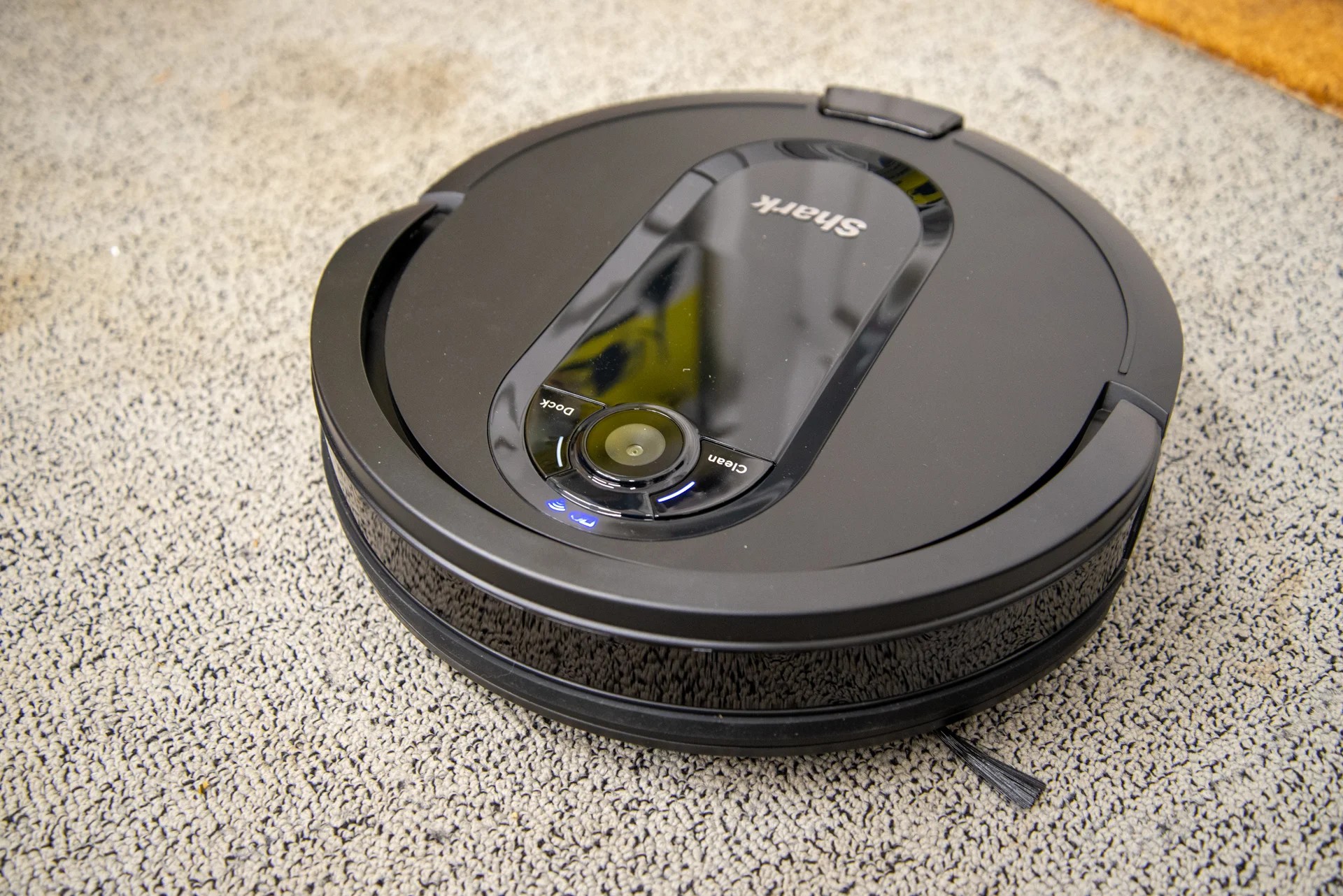
The goal of this project is to create a high-end vacuum cleaner. This cleaner would have to ensure to clean as much area as possible of a predetermined map that simulates a house. Since we are using a high-end vacuum model, we have some advantages that low-end cleaners doesn't have, such as the house map already mapped and integrated in the robot software. With this map, we can know exactly where the robot is and we can create new navigation techniques to ensure the robot cleans all the house without using random or pseudorandom cleaning skills.

First Step: Map Segmentation and interpretation

As we mentioned before, we already have the house mapped. This allow us to use covering algorithms such as Backtracking Spiral Algorithm (BSA) instead of using random or pseudorandom behavior. In order to apply this covering algorithm, we will need to transform the mapped house image into a grid map, where each cell of the map represent a coordinate (x,y) where the vacuum can be.

In order to reach a first approximation to this, I made a simple program that takes the mapped house and creates a matrix that represents each cells of the map. Notice that we can divide the map into NxM cells, but this numbers must be taken according to the robot dimensions. Is reasonable to consider that N=M (same width as height cells, this is, square cells), as the vacuum is circular. Notice in the following pictures how important is to take a reasonable cell size:

If we choose a big N number of cells, the vacuum position (x,y) > cell size, so we will be consider multiple positions for the vacuum that are overlapped (the vacuum is in more than 1 cell for a certain (x,y) position).  In the other hand, if we have a small N number of cells, the vacuum could have troubles cleaning cells that are near the occupied cells (walls or obstacles), and the cleaning performance could not be efficient.

In order to choose a correct cell size, I consider the fact that the vacuum can pass between the legs of the table (the one in the right bottom table of the map), as well as the approximated vacuum size:

Once we have chosen the right size of the grid cells, I have 2 different options to divide the cells as obstacles or free cells:

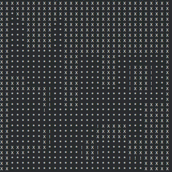
FIRST IDEA: classify the cells in 3 categories:

• OBSTACLE CELL: If the cell represents a group of pixels of the image that are entirely black (0) or it mean is less than a lower value. Lets call this value LOWER_OBSTACLE_THRESHOLD
• FREE CELL: If the cell represents a group of pixels of the image that are entirely white (255) or it mean is greater than a upper value. Lets call this value UPPER_OBSTACLE_THRESHOLD
• EDGE CELL: If the cell represents a group of pixels of the image that are between both mentioned thresholds.

After adjusting the threshold values, we had a first approximation of the real grid map that the robot would take in consider for the navigation algorithm:

SECOND IDEA: Dilate map it to increase walls and obstacles areas. Using this idea we remove the 'edge' category, Now, the cells will be only divided in 'Obstacle' cell or 'Free' cell. Using a conservative point of view to avoid problems with obstacles, using this idea we will consider 'Free' cells the ones that have all pixels white. This is, if any cell has any black pixel, it will be tagged as 'Obstacle' cell:

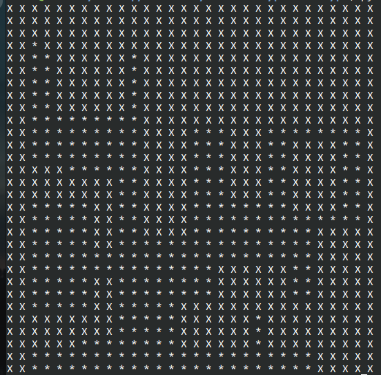
We will have in consider this second idea due to it's safety advantages with the obstacles and the reduction of cells that could end up with cleaning troubles for the vacuum.

Second Step: Localization in the grid map

The API give us the coordinates (x,y) of the robot in the 3D world, as well as the yaw (orientation). But all the logic and intelligence of the robot will have in consider the grip map, so we need to transform that coordinate and orientation system to the correspondence position in the 2D grid map.

In order to do this, we will choose a number of points in the 3D world and the (approximated) correspondent pixel in the 2D map and we will compute the best fitting regression line to do this transformation between coordinates. For this samples, we will take points that are a little bit distant between them to reduce the error. The best option is to take corner points and the origin point of the Gazebo world:

After some measures, we have the following regression line using a sample of 6 different points of the map:

This is the mathematical expression in form of y = b + m*x

With this we already have a mechanism to manage the coordinates of the vacuum. We have now totally localized our vacuum in the 2D grid map we have created, no matter the number of cells (could be changed in the next steps of the project)

NOTE: This regression lines were calculated after the bug of coordinates error of Unibotics were fixed. Before, the regression line for both pixelX and pixelY were a bit higher than now.

Third step: Navigation using BSA

Now that we have our movement primitives, its time to apply the BSA Covering Algorithm for the navigation of the vacuum. The BSA algorithm consist of a movement technique to cover the much area possible using "spirals" paths:

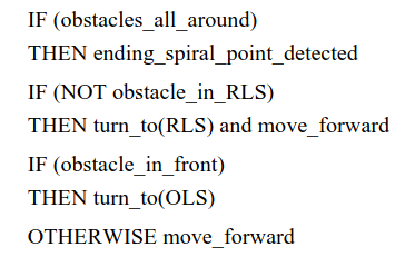
The robot starts moving in a certain direction, lets call DIR1, till he reaches the last cell in that direction that is not an obstacle. Then, he turns to a perpendicular direction, called DIR2. Again, the robot checks if he can go again to the DIR1 (if there is not obstacle in that direction), or in the contrary direction to DIR1. In some moment of the algorithm, the robot will be completly surrounded by obstacle cells or visited cells, when it will be the time for the robot to move to a "checkpoint" or "return cell point" to continue the algorithm .The result of this movements creates a spiral paths of this type:

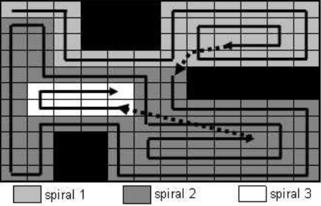
In our program, we will create a list of directions, DIRECTIONS_ORDER, following the rules we mentioned above ([DIR1, -DIR1, DIR2, -DIR2]). We will iterate from the least priority direction to the most priority looking for not visited cells. If we found one, we will store that cell both as possible return point and possible next cell to visit. Once we finish iterating all the neighbors, we will choose only the last possible cell to visit as next cell to go, and we will store the possible returning points in a list, that will increase or decrease in our program depending on if we have visited that cell or not.

Visual approximation

We will do a first approximation in our program using the Open-CV Grid-Image we created for the Inner map of the vacuum (we will not use Unibotics for this first test). First of all, we create 2 classes in our program:

• CLASS VACUUM: This class will represent the vacuum robot, and will have their own attributes: Grid position, Pixel position, angular and linear velocity and the list of returning cells where the vacuum can go when he is surrounded by obstacles/visited cells.
• CLASS CELL: Represents the cell itself, with his [x,y] position in the grid map, his boundaries in the Image (pixels), its center coordinates and also his state (Visited cell, Not visited cell or Obstacle cell).
  

Once we have the classes created, as well as the map segmentation, the localization conversion from 3D world to 2D grid map and the BSA algorithm, this is the result of a visual approximation of the solution:

Where the dark green cells represents the list of possible returning points for the robot when a spiral is finished. The light green cells are the visited ones, the red point the robot, and the white cells the not visited cells.

Notice that we have not implemented still the recovery algorithm for the vacuum to move from the last cell of the current spiral to the nearest returning cell to start the next spiral.

Fourth step: Recovery. Returning cell implementation

In order to check in Unibotics our program, we only have one missing thing to do: the recovery algorithm. When the robot finish a spiral and needs to return to the nearest returning point marked, it can happen two things:

• RETURNING POINT IS VISIBLE IN STRAIGHT LINE FROM CURRENT POSITION: The robot could just create a path in straight line, with a certain yaw, to reach the return cell.
  
• RETURNING POINT IS NOT VISIBLE IN STRAIGHT LINE FROM CURRENT POSITION: The robot needs to implement a recovery algorithm to find the best path of cells to reach the return cell.

There is no problem if we have the first case. But, if we have the second case, we need to think which navigation algorithm could be the best to find a solution to that problem.

There are many different algorithms to do this. Here is a list I though:

• VFF (Virtual Force Field): The returning cell center coordinate is the goal. This goal creates a virtual force that attracts the robot. The obstacles of the map (walls, etc...) creates an opposite force. This forces are used in a linear combination to compute an average force: F_average = alpha*F_attraction + beta*F_repulsive. This average force will be the one to follow in order to reach the return cell avoiding the obstacles of the map.
• GPP (GRADIENT PATH PLANNING): We will create a field in the returning point that expands among the map using a search algorithm without crossing the obstacles. The wave will stop when we reach the current position.
• SEARCH ALGORITHMS (INFORMED VS NO INFORMED): We can use informed algorithms that uses heuristics to find the best path, or not informed algorithms if the heuristic is not viable. The best search algorithms as Breadth First Seach (BFS), deep First Search, A*...

 In the end, I decided to use the Breadth First Seach (BFS) algorithm for this task, which can be written in pseudo-code as follow:

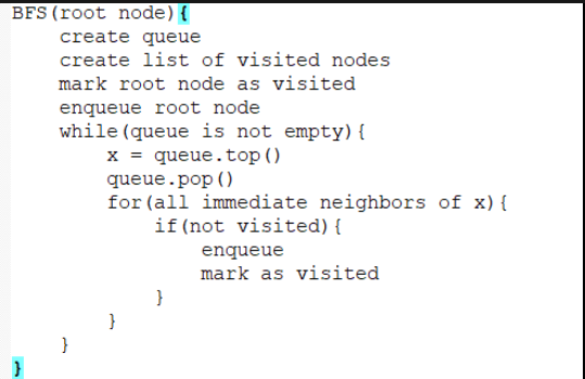
To implement this algorithm, I created in the program two new functions:

• getSuccessors(): gets the cells neighbors (x + 1, x - 1, y + 1, y - 1) of the current cell and return them if they are not obstacles and the cells have not been visited in the BFS algorithm:
• breadthFirstSearch(): Uses described algorithm above to search for the path from cell A to a cell B of the grid. Uses the getSuccessors() function.
  

Once we have implemented this algorithm, and we have tuned the movement primitives, we can try our program now and see how the robot doesn't teleport now from the end of a spiral to a nearest point. Now, the robot is able to find a path to go to the return point. Note that BFS recovery algorithm will be used always, even if it is direct visibility between the current cell and the return cell:

Fifth step: Navigation primitives

Before implementing the code in Unibotics, we have to decide what movement primitives will have our vacuum. This means how will the robot move from a specific cell center to another cell center and how will turn exactly x degrees to turn exactly right or left. Also, we will also need a mechanism to update every cell is visited, now that we have our vacuum localized in the grid map.

LINEAR MOVEMENT PRIMITIVE

In order to move in a straight line, we will just use the API command to set velocity for the vacuum. In this moment, the linear movement problem suggest to different options for the solution:

• Use a constant linear velocity for the vacuum along all the algorithm, even if its near an obstacle or too close to the last cell before turning.
  
• Use a range of velocities between [MIN_LINEAR_VEL, MAX_LINEAR_VEL]. The robot would always use the max linear velocity when it is not too close from a target cell (last cell of a straight path of cells before turning) or near any obstacle. When the vacuum is too close of the (x,y) target or < OBSTACLE_THRESHOLD value from a wall, it will slow down from its current velocity to a minimal of MIN_LINEAR_VEL value.

In order to get a first approximation, we will start using a constant linear velocity when the robot is not turning (this is, when the vacuum is orientated to the goal direction). This linear velocity will be the maximum velocity, defined as MAX_LINEAR_VEL.

Note that, for a better approach to a real scene, the best idea is to use the second option. This will allow us to gain security in the navigation algorithm and avoid hitting the break when the vacuum its about to crash on a wall or to start turning to another direction (out of this simulator, this behavior can cause issues in the robot motor).

TURNING MOVEMENT PRIMITIVE

In the other hand, we need a turn movement primitive for the vacuum. The API command that give us the yaw of the vacuum we have a range of [-π,+π] values. We need to focus on the values of exactly 0, -π/2, |π|, π/2 for the directions of WEST, NORTH, EAST and SOUTH, respectively, in order to move the vacuum exactly in that directions.

For a first and easy approximation, we will use the following concept:

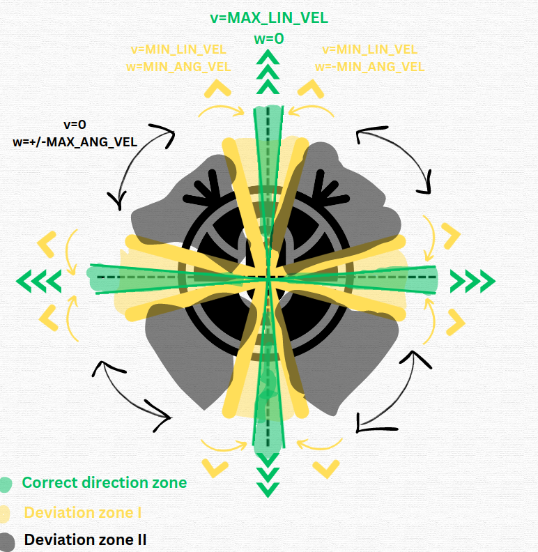
• Correct direction zone: When the error between the robot direction and the target direction is equal or less than ANGLE_ERROR_THRESHOLD. For performance reasons, this value should be small (1º or 0.02 radians). The robot will have maximum linear velocity and 0 angular velocity.
  
• Deviation zone I: When the error between the robot direction and the target direction is equal or less than ANGLE_ERROR_THRESHOLD_2. The value should be well-balance. The robot will have minimal linear velocity and minimal angular velocity in order to correct the direction.
• Deviation zone II: When the error between the robot direction and the target direction is greater than ANGLE_ERROR_THRESHOLD_2. The robot will not have linear velocity and will turn at maximal angular velocity to correct direction.

Sixth step: Configuration values and Unibotics tests

Once we have the BSA algorithm, the recovery BFS algorithm and the movement primitives, its time to check how it works the program in Unibotics. The key of this exercise is to adjust each of the constants (parameters) to a correct value, specially the following ones:

• GRID_CELLS: Number of cells to create in the inner map of the robot. Cells size must be related with the robot dimensions in order to do a good execution.
• ANGLE_ERROR_THRESHOLD: Defines the limit between correct direction zone and Deviation zone I.
  
• ANGLE_ERROR_THRESHOLD_2: Defines the limit between Deviation zone I and Deviation zone II.
  
• PIXELS_ERROR_THRESHOLD: Defines the error we can handle when checking if robot reached the goal cell center.
  
• MIN_LIN_VEL: Minimal linear velocity robot can have
  
• MAX_LIN_VEL: Maximal linear velocity robot can have
  
• MIN_ANG_VEL: Minimal angular velocity robot can have
  
• MAX_ANG_VEL: Maximal linear velocity robot can have
  
• KERNEL_IMG_SIZE: Kernel size for the morphological operation (in order to increase obstacles)
  
• MORPH_ITERATIONS: Number of iterations to do in the morphological operation (in order to increase obstacles)

FIRST WORKING VERSION

Here is the result of executing the first working version of our program for ~25 minutes, after finding reasonable values for each of the mentioned parameters:

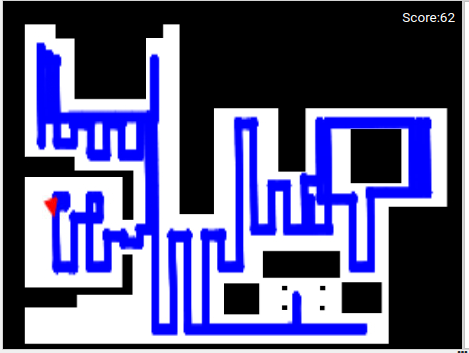
We can see that we have a considerable good cleaning in a reasonable time interval, but we can improve some things in our program to reduce, among others, the cleaning time.

SECOND WORKING VERSION

We have been calculating the path (the next cell to go) during all the program execution until now. We can change the main logic of the program and get all the path at the start of the program. If we do this, we will have the complete path (next cells to go) in a list, so we will just need to pop(0) from that list each time we reach a new objective, and don't think about who will be the next cell. In order to do this, we introduce a new function to the program, called generatePath(), that takes as argument the starting point of the map, the robot object and the grid map:

We can also improve this dynamic: we can reduce the number of goal cells and get as goal only the ones in the path that are the last ones in the current direction. This is, for example, that if we are going to follow 10 cells that are in a column, from north to south, get as goal only the last cell in that column. Notice that the chosen return cells of the algorithm are special and they can't be erased from the path when simplifying this, so we will mark them as "Special Cells", introducing a new attribute to the Cell class. The new function to apply this improve is simplifyPath(), and the idea is the following idea:

Note that, this doesn't affect when robot is changing direction (it will just pick up the next cell in the path to "orientate" to the new goal direction). With this new implementation, we will reduce the "stops" and the pop(0) operations in our program.

Another thing that can be highly improved is the velocity control. Remember we used to apply a constant linear velocity all the time, but with the reduction of goal cells, we can now apply a linear PD Controller that vary the vacuum velocity for the range [MIN_LINEAR_VEL, MAX_LINEAR_VEL], as we introduced in Step Fifth of this blog entry.

We can also apply a PD Controller to the angular velocity. Remember we used to use a 2 threshold mechanism to divide the angular velocity is Minimal, angular or null. In this new version of my program, I remove the inner threshold, and I compute now the angular velocity using a PD Controller if we are inside the remaining threshold:

In order to do that, we created the class Controller, that represents a PD Controller for both linear and angular velocities.

Note that now we have removed 2 of the previous key parameters of the list, but with the PD constants we are introducing new ones. Here is the new list of key parameters to take in count during the project:

• GRID_CELLS: Number of cells to create in the inner map of the robot. Cells size must be related with the robot dimensions in order to do a good execution.
  
• ANGLE_ERROR_THRESHOLD: Defines the limit to use the PD Controller output or to set the robot to maximal angular velocity and null linear velocity.
  
• PIXELS_ERROR_THRESHOLD: Defines the error we can handle when checking if robot reached the goal cell center.
  
• MIN_LIN_VEL: Minimal linear velocity robot can have
  
• MAX_LIN_VEL: Maximal linear velocity robot can have
  
• MAX_ANG_VEL: Maximal linear velocity robot can have
  
• KERNEL_IMG_SIZE: Kernel size for the morphological operation (in order to increase obstacles)
  
• MORPH_ITERATIONS: Number of iterations to do in the morphological operation (in order to increase obstacles)
• KP: Proportional constant of the controller (there's one for the linear and another for the angular)
• KD: Derivative constant of the controller (there's one for the linear and another for the angular)
  

With this new update, we have:

• Increased efficiency: Our program do less computing work in each of the iterations, the main loop simplifies and the code looks more simple.
• Reduce cleaning time: Using a linear velocity that depends on the goal distance allow us to increment the previous MAX_LINEAR_VEL. Also, using continuous values for the angular velocity allow us to slightly correct better the direction due to some oscillations (specially now that the robot can move faster). The vacuum will clean faster than before, increasing considerably the precision and reducing the errors.

Let's try out the new version of the program and see if we are right with the previous points . Here is the result of the cleaning house after 20 minutes of work:

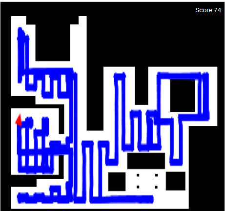
Here is a demonstration video (x8 speed):

IMPORTANT NOTE: This video has been recorded using Unibotics in local mode. The performance due to my computer is not good, and the gazebo simulator starts to get a lot of lag at the mid time of the video. The video has been speed up x8, but the RTF was about 0.65 from the start to the mid time of the video, and then the RTF decreases significantly. The estimated cleaning time of the robot is around ~22 minutes (tested in remote mode).